Complex systems require complex logic. When you design software, embedded controllers, or workflow engines, simple linear flows often fall short. You need a model that captures simultaneous behaviors without cluttering the visual representation. This is where the concept of orthogonal regions in UML state machine diagrams becomes essential.
State diagrams are powerful tools for modeling reactive systems. However, as requirements grow, the diagram can become a tangled web of transitions. Orthogonal regions offer a structured way to handle concurrency. They allow a single state to contain multiple independent sub-states that evolve in parallel. This guide provides a deep dive into how these regions function, why they matter, and how to apply them effectively in your modeling efforts.
What Are Orthogonal Regions? ⚙️
In the context of the Unified Modeling Language (UML), an orthogonal region is a partition within a composite state. The term “orthogonal” implies independence. Two dimensions are orthogonal if they do not interfere with each other. In state modeling, this means two different aspects of a system’s behavior can operate simultaneously.
Imagine a composite state as a container. Inside this container, you can draw lines to divide the space into separate areas. Each area is a region. Transitions within one region do not directly affect the transitions in another region, unless explicitly connected by shared events or synchronization.
Key characteristics include:
Concurrency: Multiple regions are active at the same time.
Independence: Logic in one region runs without blocking another.
Composition: They exist only inside a composite (nested) state.
Visual Separation: Drawn with a dashed or solid line dividing the parent state.
Without orthogonal regions, you might be forced to model these behaviors as separate top-level states or create a massive state with excessive branching. Orthogonal regions keep the model clean and the logic modular.
Visualizing the Structure 📊
To understand how this looks in practice, consider the notation used in UML specifications. A composite state is typically a rounded rectangle. When you introduce orthogonality, you divide this rectangle into sub-regions.
Here is how the structure breaks down:
Parent State: The enclosing composite state.
Region Divider: A line splitting the parent state.
Child States: States located within each specific region.
Initial Pseudo-State: Each region typically starts with a filled circle indicating the entry point.
When the parent state is entered, all initial states in all regions are activated simultaneously. When the parent state is exited, all active child states must be exited first.
Why Use Orthogonal Regions? 🎯
Modeling systems is about reducing cognitive load. If you can represent complex behavior with a clear diagram, the implementation becomes easier to reason about. Here are the primary reasons to adopt this pattern:
1. Handling Concurrency Naturally
Many systems have parts that run at the same time. A security system might monitor alarms while simultaneously tracking the time. A database might handle queries while logging transactions. Without orthogonal regions, you would have to create a flat state with every combination of these conditions (Alarm On + Time Active, Alarm Off + Time Active, etc.). This leads to combinatorial explosion.
2. Modularity and Reusability
By separating concerns into different regions, you isolate logic. If the “Time Tracking” logic changes, you only modify that region. The “Security Monitoring” region remains untouched. This separation of concerns is a core principle of software architecture.
3. Clarity in State Representation
A single composite state with orthogonal regions is often smaller and clearer than a flat state machine with hundreds of transitions. It groups related behaviors under a single umbrella while maintaining their independence.
Deep Dive: A Practical Example 🏠
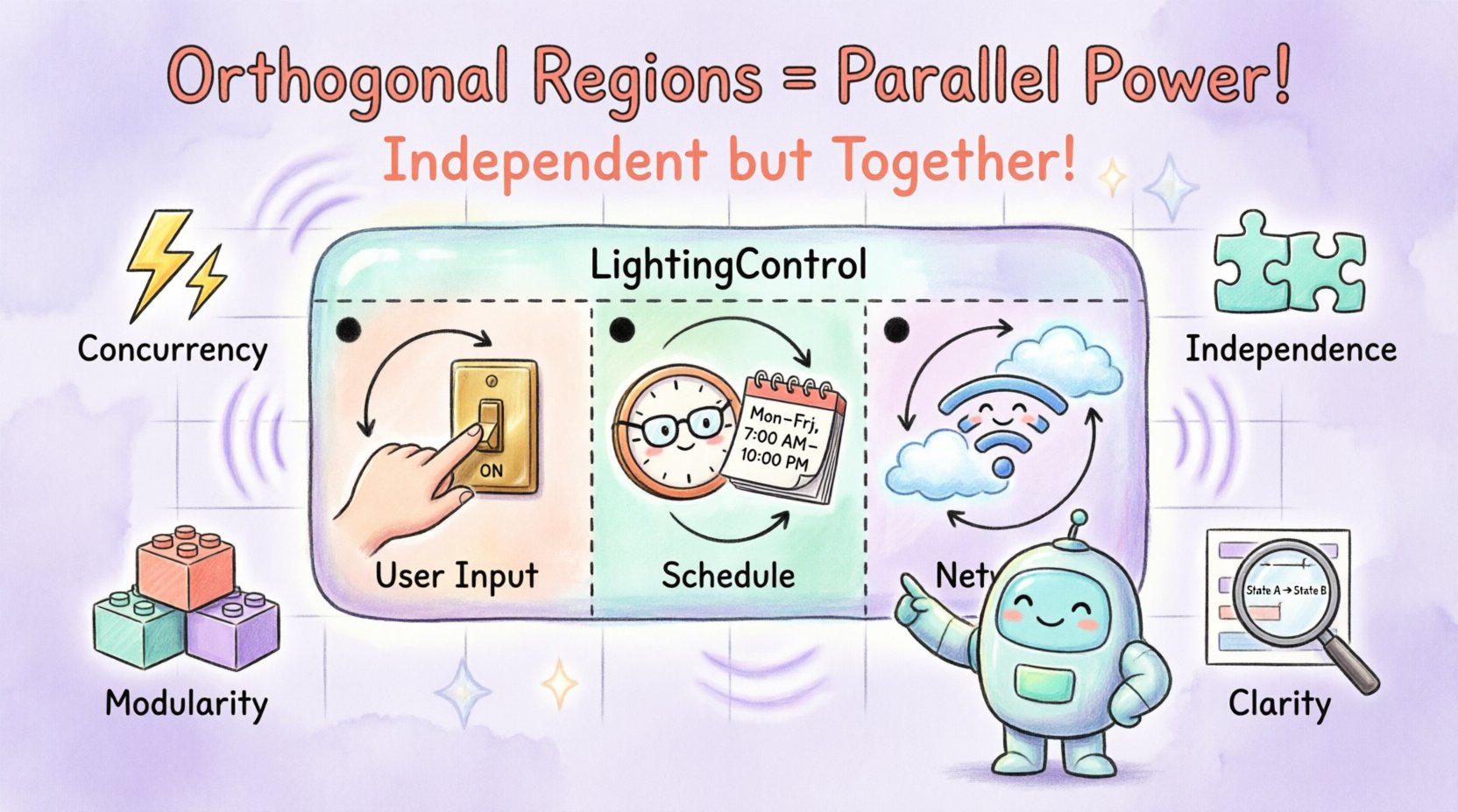
Let us construct a scenario. Consider a Smart Home Lighting Controller. This device needs to manage lighting based on user input and automatic scheduling.
Here are the conflicting requirements:
The system must react to manual switches (User Override).
The system must follow a schedule (Auto Mode).
The system must report status to the network (Connectivity).
If we model this as a single flat state machine, we would need states for “Manual On”, “Manual Off”, “Schedule On”, “Schedule Off”, “Offline Manual On”, “Offline Manual Off”, etc. This is inefficient.
Instead, we define a composite state called LightingControl. Inside, we create three orthogonal regions:
Region A (User Input): Handles switch toggles.
Region B (Schedule): Handles time-based rules.
Region C (Network): Handles Wi-Fi status and updates.
When the LightingControl state is active, all three regions are active. The user can toggle a switch (Region A) regardless of what the schedule (Region B) is doing. If the Wi-Fi drops (Region C), the manual override (Region A) still works.
State Transition Logic
How do these regions interact? They typically do not interact unless specified. However, the final output (Light On vs. Light Off) is determined by the combination of these regions.
We can define a rule:
If User Input is “On”, Light is “On”.
Else, if Schedule is “On”, Light is “On”.
Else, Light is “Off”.
This logic is implemented in the system code, not the diagram. The diagram simply shows that the system maintains these three independent contexts simultaneously.
Comparing Region Types 📋
Not all nested states are orthogonal. It is crucial to distinguish between hierarchical nesting and orthogonal partitioning. The following table clarifies the differences.
Feature | Orthogonal Regions | Sequential States | History States |
|---|---|---|---|
Execution | Parallel | One at a time | Restores previous state |
Dependency | Independent | Dependent on parent | Dependent on exit |
Entry Point | Multiple initial states | Single entry path | Shallow or Deep |
Use Case | Concurrency (e.g., Clock + Alarm) | Phased processes (e.g., Login Flow) | Returning from interruption |
Visual | Divided rectangle | Nested rectangle | Arrow with “H” marker |
Understanding these distinctions prevents modeling errors. If you put states in a sequential flow inside a composite state, you force them to run one after another. If you put them in orthogonal regions, they run together.
Entry and Exit Actions 🔄
One of the most critical aspects of managing orthogonal regions is handling entry and exit actions. Because multiple regions are active simultaneously, the timing of these actions matters.
Entry Actions
When a composite state is entered:
All initial pseudo-states in all regions are triggered.
Entry actions defined on the composite state itself run first.
Entry actions on the specific child states run next.
Consider a Medical Patient Monitor. The composite state is Monitoring. It has two regions: Vitals and Alarms.
Composite Entry: Initialize system clock.
Vitals Entry: Start sensor polling.
Alarms Entry: Load threshold limits.
All these happen when the Monitoring state begins. If you need to sequence them, you must use transitions between child states within the regions, not rely on the entry mechanism alone.
Exit Actions
When leaving the composite state, the order of exit is generally:
All active child states in all regions must be exited.
Exit actions on the child states run.
Exit actions on the composite state run.
If one region enters a state that cannot exit immediately (e.g., waiting for a network response), the entire composite state remains active. This is a critical synchronization point for developers.
History States and Orthogonality 🧠
History states are used to remember the previous state within a composite region. When combined with orthogonal regions, they become powerful but require careful management.
There are two types of history:
Shallow History (H): Remembers the last active state within the immediate composite state.
Deep History (⊗): Remembers the last active state within the entire hierarchy of nested states.
In an orthogonal setup, each region maintains its own history. If Region A has a history state, it remembers where it was in Region A. Region B has its own history, independent of Region A.
Scenario: Emergency Vehicle System
Region 1: Radio Communication (History: Last frequency).
Region 2: Siren Control (History: Last mode).
If the system pauses and resumes, Region 1 restores the radio frequency, and Region 2 restores the siren mode. They do not interfere with each other. This independence is the primary benefit of using history states alongside orthogonal regions.
Common Pitfalls and Mistakes 🚫
Even experienced modelers struggle with orthogonal regions. Here are the most frequent issues encountered during implementation and design.
1. The Synchronization Trap
It is tempting to assume regions are completely isolated. However, they share the same system clock and event queue. If Region A emits an event and Region B listens, they are synchronized by that event.
Problem: If Region A sends a signal to Region B, but Region B is currently in a state that ignores that signal, the signal is lost.
Solution: Always define how events are broadcast. Ensure critical states in listening regions are designed to handle events from any time.
2. State Explosion in Logic
Just because you can model it in parallel doesn’t mean the code should be. If the logic in Region A depends heavily on Region B, you might be creating a tight coupling that looks like concurrency but behaves like a sequence.
Problem: Code becomes hard to test because you need to mock both regions.
Solution: Review the dependency graph. If Region A cannot run without Region B being in State X, consider if a composite state hierarchy is better than orthogonal regions.
3. Entry Point Confusion
Each region must have exactly one initial pseudo-state. It is a common error to have multiple entry points or no entry points in a region.
Problem: The state machine becomes undefined on entry.
Solution: Verify that every region has a single filled circle indicating where execution begins when the parent enters.
4. Race Conditions
In software implementation, if two regions update a shared variable simultaneously, you risk a race condition. The diagram shows logical concurrency, but the code executes on a single thread or scheduler.
Problem: Data corruption or unexpected state values.
Solution: Implement locking mechanisms or use a state management pattern that serializes access to shared resources.
Implementation Considerations 💻
Translating a UML diagram with orthogonal regions into code requires a specific architecture. You cannot simply write a giant switch-case statement.
State Machine Engines
Modern development often utilizes state machine engines. These libraries handle the orthogonal logic automatically. They maintain a context for each region.
Context: A data structure holding the current state and history.
Queue: Events are queued and processed per region or globally.
Transition Table: Defines valid moves from one state to another.
Event Broadcasting
When an event occurs, the engine checks all regions. It determines which region owns the current state and processes the transition there. If the event is relevant to another region, it is propagated.
Error Handling
What happens if a transition fails in one region? In a strict system, the entire composite state might need to transition to an error state. In a robust system, only the affected region resets.
Design your error handling strategy early. Decide if the system is “fail-safe” (stops everything) or “fail-operational” (isolates the error).
Advanced Patterns: Hierarchical Orthogonality
You can nest orthogonal regions inside other composite states. This is valid in UML but should be used sparingly.
When to Nest
When a subsystem has its own independent parallel behaviors.
When you need to group orthogonal regions under a higher-level management state.
Example: Drone Flight Control
Consider a drone. The main state is Flight. Inside Flight, there is a sub-composite state called Stabilization. Inside Stabilization, you have orthogonal regions for Roll and Pitch.
Outside of Stabilization, you have another orthogonal region for GPS Tracking.
This creates layers of concurrency. The Roll and Pitch are tightly coupled (both part of stabilization), while GPS is independent. This hierarchy helps manage complexity by grouping related parallel tasks.
Testing the Model 🧪
Verifying a state machine with orthogonal regions is more complex than a linear flow. You need to cover the interaction of states across regions.
State Coverage: Ensure every state in every region is visited.
Transition Coverage: Ensure every transition between states is triggered.
Concurrent Coverage: Test scenarios where two regions change state simultaneously.
Event Ordering: Test what happens if Event A arrives before Event B versus after.
Automated testing tools can parse the UML model and generate test cases for these paths. This ensures the implementation matches the design.
Best Practices for Clarity 🌟
To keep your models maintainable, follow these guidelines:
Limit the Number of Regions: Two or three regions are usually sufficient. More than three makes the diagram hard to read.
Use Meaningful Names: Name regions by their function, not by their position. Use “Audio” instead of “Region 1”.
Document Interactions: If regions communicate, draw the connection explicitly or add a note explaining the protocol.
Keep Regions Balanced: If one region has 50 states and another has 2, reconsider the split. It suggests the first region might need to be its own top-level state.
Clarity in the diagram leads to clarity in the code. If a developer cannot understand the state flow in five minutes, the model is too complex.
Summary of Key Takeaways 📝
Orthogonal regions are a fundamental feature of UML state machine diagrams. They enable the modeling of concurrent behaviors within a single state context. By dividing a composite state into independent regions, you can represent systems that perform multiple tasks simultaneously without creating a tangled web of transitions.
Key points to remember:
Orthogonal regions run in parallel.
Each region has its own entry and exit points.
They promote modularity and separation of concerns.
Implementation requires careful handling of shared events and resources.
History states work independently within each region.
When applied correctly, this pattern reduces the complexity of your system design. It allows you to focus on the logic of individual components while maintaining a high-level view of the system’s overall state. Mastering this concept leads to more robust, maintainable, and scalable software architectures.
As you design your next state machine, ask yourself: Are these behaviors truly sequential, or can they run side by side? If they can run side by side, orthogonal regions are the path forward.