Sequence diagrams form a cornerstone of system design documentation. They provide a visual representation of interactions between objects over time. While often used to show simple call chains, their true power lies in the ability to model complex timing constraints and internal state transitions. This guide explores the mechanics behind message flow, timing analysis, and how state changes are represented within the lifelines of a system.
Understanding these diagrams requires more than just knowing the syntax. It demands an appreciation for how time flows through a system and how objects transition from one condition to another. Whether you are designing a distributed system or refining an existing architecture, clarity in these diagrams prevents ambiguity during implementation.
Core Components of a Sequence Diagram 🧩
Before diving into timing and state, it is essential to establish a shared vocabulary. Every diagram is built from specific elements that convey meaning.
- Lifelines: Vertical dashed lines representing the existence of an object or participant throughout the interaction. They define the temporal scope of the entity.
- Activation Bars: Rectangular boxes on a lifeline indicating when the object is actively performing an action or is in the process of executing a method.
- Messages: Horizontal arrows connecting lifelines. They represent the communication between objects.
- Return Messages: Dashed arrows pointing back from the receiver to the sender, indicating the completion of a task.
- Combined Fragments: Frames that group interactions to denote logic like loops, alternatives, or parallel processes.
Each of these elements contributes to the narrative of the system. When analyzing timing, the length and position of activation bars become critical indicators of system performance and bottlenecks.
Analyzing Message Timing ⏱️
Time is the defining dimension of a sequence diagram. Unlike class diagrams which show static structure, sequence diagrams depict dynamic behavior. Analyzing timing involves understanding the duration of operations and the synchronization points between components.
Types of Messages and Their Timing Implications
Different arrow styles denote different behaviors, which directly impact how time is spent in the system.
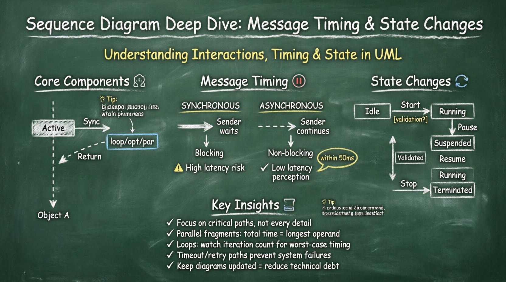
- Synchronous Messages: The sender waits for the receiver to finish the operation before continuing. This creates a blocking point in the timeline.
- Asynchronous Messages: The sender sends the message and continues immediately without waiting for a response. This allows for parallel processing.
- Return Messages: These indicate the flow of data back to the caller. They do not typically block the sender unless the logic requires the data to proceed.
- Self-Call: An object invoking a method on itself. This is often used to represent complex internal processing that takes time.
When modeling high-concurrency systems, distinguishing between synchronous and asynchronous calls is vital. A synchronous chain can create a bottleneck if any single step is slow. Asynchronous flows allow the system to remain responsive while background tasks complete.
Timing Constraints and Delays
Sometimes, the exact duration of an operation is irrelevant, but the timing relative to other events is critical. Timing constraints allow modelers to specify these relationships.
- Time Intervals: You can specify that a message must arrive within a certain timeframe (e.g., “within 50ms”).
- Periodic Messages: Used in monitoring or heartbeat systems where events occur at regular intervals.
- Delay Boxes: Represented by a small box on the activation bar, indicating a pause in processing.
Consider a scenario where a user action triggers a database query. If the database is slow, the activation bar on the database lifeline will extend. If the system is designed to be asynchronous, the user interface lifeline will continue to process other requests while waiting for the response.
Timing Analysis Table
| Message Type | Blocking Behavior | Use Case | Timing Impact |
|---|---|---|---|
| Synchronous | Yes | Immediate Data Retrieval | High Latency Risk |
| Asynchronous | No | Background Processing | Low Latency Perception |
| Self-Call | N/A | Internal Logic | Processing Depth |
| Return | Optional | Data Confirmation | Network Overhead |
Tracking State Changes Within Lifelines 🔄
State changes are the internal transitions of an object. While sequence diagrams focus on interactions, they also reveal the lifecycle of objects. An object moves through various states (e.g., Idle, Processing, Completed, Error) during its existence.
Representing State Transitions
State transitions are often implied by the messages received and the resulting activation bars. However, explicit state modeling can clarify complex logic.
- Entry and Exit Points: Indicate when an object enters a specific state upon receiving a message.
- Guard Conditions: Logic checks that determine if a transition can occur. These are often noted near message arrows.
- State Boxes: Some modeling approaches allow placing state boxes on the lifeline to show the object’s status at a specific point in time.
For example, consider an order processing system. An Order object might start in a “Created” state. Upon receiving a “Validate” message, it transitions to “Validated”. If validation fails, it moves to “Rejected”. These transitions dictate which subsequent messages are valid.
State Machine Integration
While sequence diagrams show the flow of messages, state machines show the allowed states. In advanced design, these two diagrams are used in tandem. The sequence diagram shows the external triggers, while the state machine defines the internal rules.
When a message arrives, the object checks its current state. If the state allows the transition, the message is processed. If not, the message might be ignored or trigger an error state. This prevents invalid operations and ensures data integrity.
State Change Table
| Current State | Trigger Message | Resulting State | Side Effect |
|---|---|---|---|
| Idle | Start Request | Running | Resource Allocation |
| Running | Pause Request | Suspended | Context Save |
| Suspended | Resume Request | Running | Context Restore |
| Running | Stop Request | Terminated | Resource Release |
Combined Fragments and Logic Flows 📊
Real-world systems are rarely linear. They involve loops, conditional branches, and parallel threads. Combined fragments allow the sequence diagram to capture this complexity without becoming a tangled web of arrows.
Loops and Iterations
When a process repeats, a loop fragment is used. This is common in data processing or polling mechanisms. The loop condition defines how many times the interaction occurs.
- Loop: Indicates repeated execution until a condition is met.
- Opt: Represents optional interaction, useful for error handling or conditional logic.
Timing analysis becomes more complex here. A loop can significantly extend the duration of the interaction. It is important to note the maximum number of iterations to estimate worst-case timing scenarios.
Parallel Processes
Some systems operate concurrently. Parallel fragments show that multiple lifelines are active at the same time. This is crucial for understanding resource contention.
- Par: Indicates parallel execution. All operands execute simultaneously.
- Concurrent Timing: The total time for a parallel fragment is determined by the longest operand, not the sum of all operands.
For instance, a web server might handle multiple requests simultaneously. The sequence diagram would show parallel activation bars on the server lifeline. This visualizes the capacity of the system to handle load.
Interaction Overview
When diagrams become too large, they can be broken down into interaction overview diagrams. These act as a high-level map, pointing to specific sequence diagrams for detailed views. This modular approach keeps the timing analysis focused.
Common Pitfalls and Optimization 🛠️
Even experienced modelers make mistakes that obscure the true behavior of the system. Recognizing these patterns helps in creating clearer documentation.
- Too Many Lifelines: If a diagram has too many participants, it becomes unreadable. Group related objects or use interaction overview diagrams.
- Unclear Timing: If the distance between messages is inconsistent, it implies timing differences that may not exist. Keep the layout consistent.
- Mixing State and Behavior: Do not try to show every state transition in a sequence diagram. Focus on the critical paths that trigger state changes.
- Ignoring Return Messages: Omitting return messages can make it unclear when a process actually completes. This affects timing analysis.
Optimization Strategies
To improve the utility of these diagrams, apply the following strategies:
- Focus on Critical Paths: Highlight the most important user flows. Secondary flows can be documented elsewhere.
- Use Standard Notations: Adhere to standard UML conventions to ensure consistency across the team.
- Regular Reviews: Diagrams degrade over time as the system changes. Schedule regular reviews to update them.
- Automate Where Possible: Generate diagrams from code where feasible to ensure they match the actual implementation.
Advanced Timing Considerations ⚡
In high-performance systems, micro-optimizations in timing can matter. This section covers advanced concepts relevant to system architects.
Latency vs. Throughput
Sequence diagrams can illustrate the difference between latency (time to complete one task) and throughput (number of tasks completed over time). A diagram showing a single request highlights latency. A diagram showing parallel requests highlights throughput capacity.
- Latency Analysis: Look at the longest path from start to finish. This is the critical path for response time.
- Throughput Analysis: Look at the width of the activation bars. Wide bars indicate high resource usage, which might limit throughput.
Timeout and Retry Logic
Network failures are inevitable. Sequence diagrams should include paths for timeouts and retries. This ensures that the system’s resilience is documented.
- Timeout: A message is sent, but no response is received within a set time. This triggers an error path.
- Retry: The system attempts the operation again. This adds complexity to the timing analysis.
Documenting these paths helps developers implement robust error handling. It also sets expectations for users regarding how long they might wait before a failure is reported.
Conclusion on Sequence Diagram Utility 📝
Sequence diagrams are more than just pictures of arrows. They are tools for reasoning about time, state, and interaction. By carefully analyzing message timing and state changes, teams can identify potential bottlenecks and design more resilient systems.
When used correctly, these diagrams bridge the gap between abstract requirements and concrete implementation. They force the team to consider what happens when things go wrong, not just when they go right. This foresight reduces technical debt and improves system reliability.
Adopting a disciplined approach to creating and maintaining these diagrams ensures that the documentation remains a valuable asset throughout the lifecycle of the software. Focus on clarity, accuracy, and the specific timing constraints that matter to your specific architecture.